Distributed System - Partitioning

This is a skimmed version of Chapter 6 ‘Partitioning’ from the book design_data_intensive_applications. I would recommend you to first read the whole chapter and use these notes for revision purpose only.

Introduction

• For very large datasets, or very high query throughput, that is not sufficient: we need to break the data up into partitions, also known as sharding.

• The main reason for wanting to partition data is scalability

• Partitioning and Replication

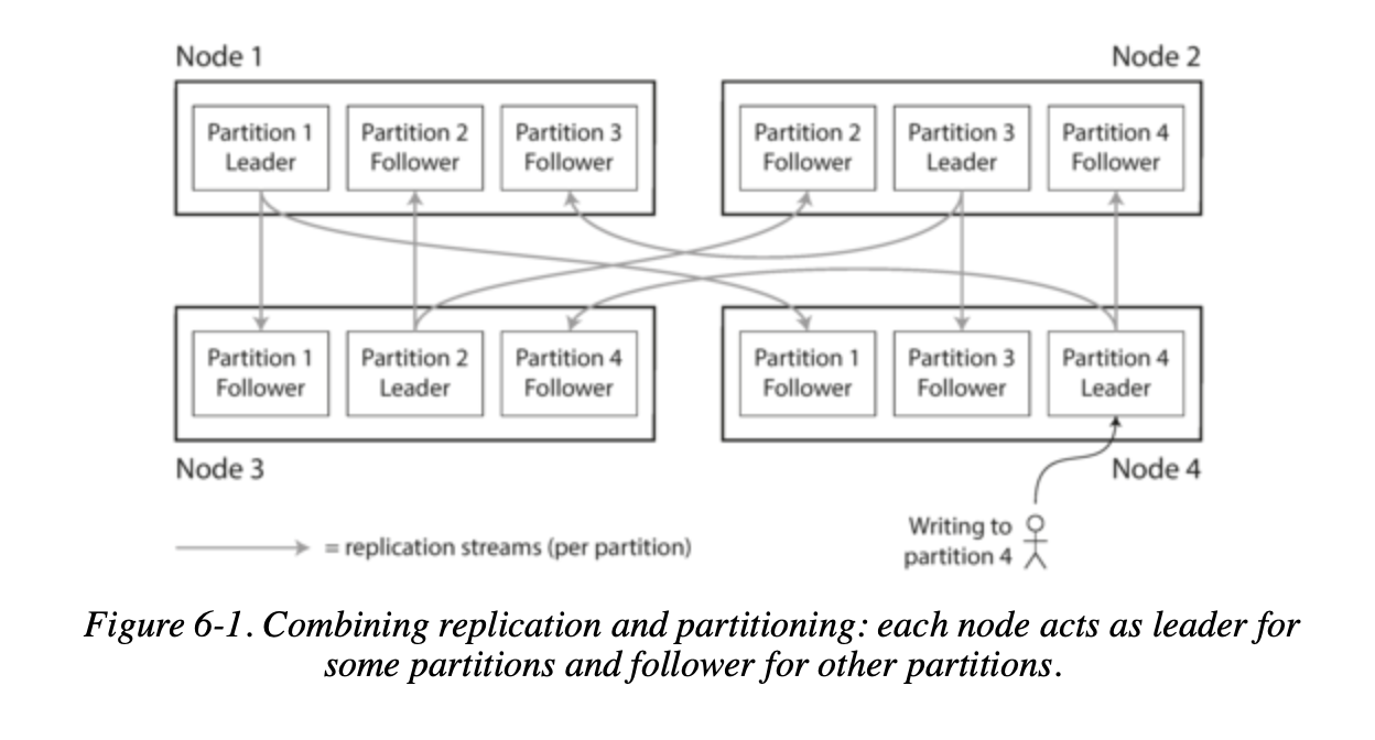
  • Partitioning is usually combined with replication so that copies of each partition are stored on multiple nodes.
  • This means that, even though each record belongs to exactly one partition, it may still be stored on several different nodes for fault tolerance.

Partitioning of Key-Value Data

• Our goal with partitioning is to spread the data and the query load evenly across nodes.
• If every node takes a fair share, then—in theory—10 nodes should be able to handle 10 times as much data and 10 times the read and write throughput of a single node (ignoring replication for now).
• If the partitioning is unfair, so that some partitions have more data or queries than others, we call it skewed.

In an extreme case, all the load could end up on one partition, so 9 out of 10 nodes are idle and your bottleneck is the single busy node. A partition with disproportionately high load is called a hot spot.

• The simplest approach for avoiding hot spots would be to assign records to nodes randomly.
• That would distribute the data quite evenly across the nodes, but it has a big disadvantage: when you’re trying to read a particular item, you have no way of knowing which node it is on, so you have to query all nodes in parallel.

Partitioning by Key Range

• One way of partitioning is to assign a continuous range of keys (from some minimum to some maximum) to each partition, like the volumes of a paper encyclopedia.
• If you know the boundaries between the ranges, you can easily determine which partition contains a given key.
• If you also know which partition is assigned to which node, then you can make your request directly to the appropriate node (or, in the case of the encyclopedia, pick the correct book off the shelf).

The ranges of keys are not necessarily evenly spaced, because your data may not be evenly distributed.

• Within each partition, we can keep keys in sorted order SSTables and LSM-Trees.
• This has the advantage that range scans are easy, and you can treat the key as a concatenated index in order to fetch several related records in one query.

Downside of Key Range Partitioning

• Certain access patterns can lead to hot spots.
  • If the key is a timestamp, then the partitions correspond to ranges of time—e.g., one partition per day.
  • Unfortunately, because we write data from the sensors to the database as the measurements happen, all the writes end up going to the same partition (the one for today), so that partition can be overloaded with writes while others sit idle.

Partitioning by Hash of Key

• Because of this risk of skew and hot spots, many distributed datastores use a hash function to determine the partition for a given key.

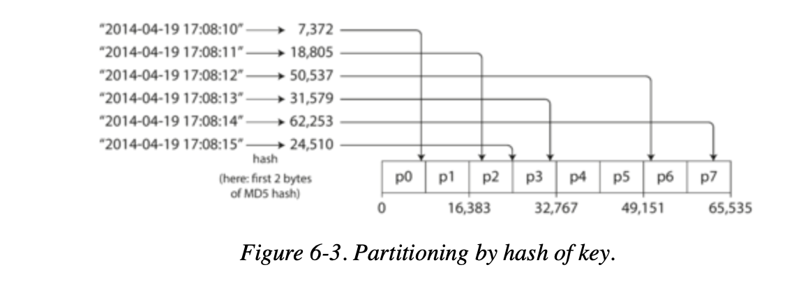
• A good hash function takes skewed data and makes it uniformly distributed.

  • Say you have a 32-bit hash function that takes a string. Whenever you give it a new string, it returns a seemingly random number between 0 and 2^32-1

• Once you have a suitable hash function for keys, you can assign each partition a range of hashes (rather than a range of keys), and every key whose hash falls within a partition’s range will be stored in that partition.

The partition boundaries can be evenly spaced, or they can be chosen pseudorandomly (in which case the technique is sometimes known as consistent hashing).

Downsides of Hash Partitioning

• We lose a nice property of key-range partitioning: the ability to do efficient range queries. Keys that were once adjacent are now scattered across all the partitions, so their sort order is lost.
• In MongoDB, if you have enabled hash-based sharding mode, any range query has to be sent to all partitions

Range queries on the primary key are not supported by Riak, Couchbase or Voldemort.

Skewed Workloads and Relieving Hot Spots

• Hashing a key to determine its partition can help reduce hot spots.

• However, it can’t avoid them entirely: in the extreme case where all reads and writes are for the same key, you still end up with all requests being routed to the same partition.

• This kind of workload is perhaps unusual, but not unheard of: for example, on a social media site, a celebrity user with millions of followers may cause a storm of activity when they do something.

• This event can result in a large volume of writes to the same key (where the key is perhaps the user ID of the celebrity, or the ID of the action that people are commenting on).

• Hashing the key doesn’t help, as the hash of two identical IDs is still the same.

• If one key is known to be very hot, a simple technique is to add a random number to the beginning or end of the key. Just a two-digit decimal random number would split the writes to the key evenly across 100 different keys, allowing those keys to be distributed to different partitions.

• However, having split the writes across different keys, any reads now have to do additional work, as they have to read the data from all 100 keys and combine it.

Partitioning and Secondary Indexes

• Partitioning schemes based on key-value data models simplify routing requests.
• However, incorporating secondary indexes complicates this, as they allow searching for values rather than just accessing records via primary keys.
• Secondary indexes are the bread and butter of relational databases, and they are common in document databases too.
• The problem with secondary indexes is that they don’t map neatly to partitions.
• There are two main approaches to partitioning
  • Partitioning Secondary Indexes by Document
  • Partitioning Secondary Indexes by Term

Partitioning Secondary Indexes by Document

• Imagine running a website for selling used cars.
• Each car listing has a unique document ID.
• Partition the database based on document ID ranges.
• Implement secondary indexes for color and make.
• The database automatically updates these indexes.
• Each partition independently manages its indexes.
• Write operations only affect the relevant partition.
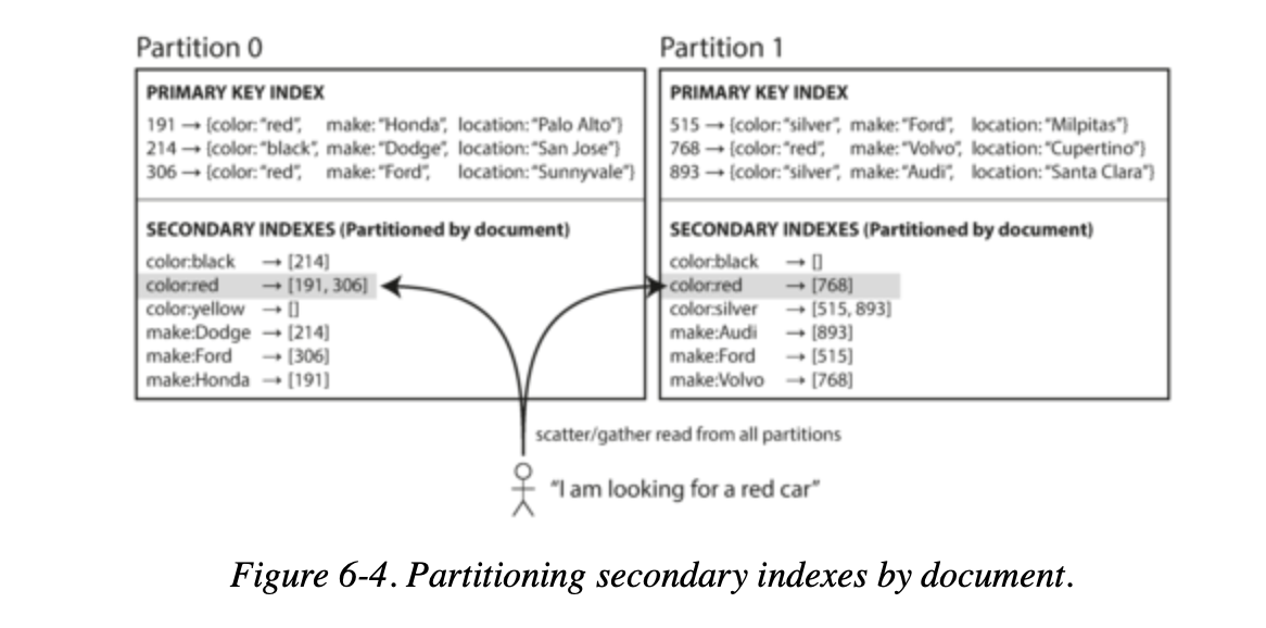
• For instance, when adding a red car, its ID is added to the color index.
• This approach is termed local indexing, differing from global indexing.

Riak, Cassandra, Elasticsearch, SolrCloud and VoltDB all use document-partitioned secondary indexes.

Downsides of Partitioning Secondary Indexes by Document

• If you want to search for red cars, you need to send the query to all partitions, and combine all the results you get back.
• This approach to querying a partitioned database is sometimes known as scatter/gather, and it can make read queries on secondary indexes quite expensive.
• Even if you query the partitions in parallel, scatter/gather is prone to tail latency amplification.

Partitioning Secondary Indexes by Term

• Rather than each partition having its own secondary index (a local index), we can construct a global index that covers data in all partitions.

• However, we can’t just store that index on one node, since it would likely become a bottleneck and defeat the purpose of partitioning.

• A global index must also be partitioned, but it can be partitioned differently from the primary key index.

• Figure illustrates what this could look like: red cars from all partitions appear under color:red in the index, but the index is partitioned so that color starting with the letters a to r appear in partition 0 and colors starting with s to z appear in partition 1.

• The index on the make of car is partitioned similarly (with the partition boundary being between f and h).

We call this kind of index term-partitioned, because the term we’re looking for determines the partition of the index.

Pros and Cons of Partitioning Secondary Indexes by Term

• The advantage of a global (term-partitioned) index over a document-partitioned index is that it can make reads more efficient: rather than doing scatter/gather over all partitions, a client only needs to make a request to the partition containing the term that it wants.
• However, the downside of a global index is that writes are slower and more complicated, because a write to a single document may now affect multiple partitions of the index (every term in the document might be on a different partition, on a different node).

Rebalancing Partitions

• Over time, things change in a database:

  • The query throughput increases, so you want to add more CPUs to handle the load.
  • The dataset size increases, so you want to add more disks and RAM to store it.
  • A machine fails, and other machines need to take over the failed machine’s responsibilities.

• All of these changes call for data and requests to be moved from one node to another. The process of moving load from one node in the cluster to another is called rebalancing.

• Rebalancing is usually expected to meet some minimum requirements:

  • After rebalancing, the load (data storage, read and write requests) should be shared fairly between the nodes in the cluster.
  • While rebalancing is happening, the database should continue accepting reads and writes.
  • No more data than necessary should be moved between nodes, to make rebalancing fast and to minimize the network and disk I/O load.

Strategies for Rebalancing

• There are a few different ways of assigning partitions to nodes.

How not to do it: hash mod N

• If it’s best to divide the possible hashes into ranges and assign each range to a partition (e.g., assign key to partition 0 if 0 ≤ hash(key) < b0, to partition 1 if b0 ≤ hash(key) < b1, etc.).
• Then why we don’t just use mod (the % operator in many programming languages).
• The problem with the mod N approach is that if the number of nodes N changes, most of the keys will need to be moved from one node to another.
  • For example, say hash(key) = 123456.
  • If you initially have 10 nodes, that key starts out on node 6 (because 123456 mod 10 = 6).
  • When you grow to 11 nodes, the key needs to move to node 3 (123456 mod 11 = 3), and when you grow to 12 nodes, it needs to move to node 0 (123456 mod 12 = 0).
• Such frequent moves make rebalancing excessively expensive.

Fixed number of partitions

• There is a fairly simple solution: create many more partitions than there are nodes, and assign several partitions to each node.

• For example, a database running on a cluster of 10 nodes may be split into 1000 partitions from the outset so that approximately 100 partitions are assigned to each node.

• Now, if a node is added to the cluster, the new node can steal a few partitions from every existing node until partitions are fairly distributed once again

• Only entire partitions are moved between nodes. The number of partitions does not change, nor does the assignment of keys to partitions.

• The only thing that changes is the assignment of partitions to nodes.

  • This change of assignment is not immediate—it takes some time to transfer a large amount of data over the network—so the old assignment of partitions is used for any reads and writes that happen while the transfer is in progress.

This approach to rebalancing is used in Riak ,Elasticsearch, Couchbas, and Voldemort.

• DOWNSIDE OF FIXED NUMBER OF PARTITIONS

  • The downside of this approach is that the number of partitions is fixed, so if you initially choose too few partitions, you may need to re-shard your database (i.e., change the number of partitions) at some point in the future.
  • Re-sharding is a difficult operation, because it requires moving a large amount of data between nodes, and it may require downtime or at least a period of reduced availability.

Dynamic partitioning

• An alternative approach is to start with a small number of partitions and partition the data dynamically.
• When a node becomes too hot, you can split one of its partitions in two, and move one of the halves to a new node.
• When a node becomes too cold, you can merge two of its partitions.
• This approach is more flexible than fixed partitioning, but it requires more sophisticated algorithms to decide when and how to move partitions.

An advantage of dynamic partitioning is that the number of partitions adapts to the total data volume. HBase and MongoDB allow an initial set of partitions to be configured on an empty database (this is called pre-splitting).

Partitioning proportionally to nodes

With dynamic partitioning, the number of partitions is proportional to the size of the dataset. On the other hand, with a fixed number of partitions, the size of each partition is proportional to the size of the dataset.

• A third option, used by Cassandra and Ketama, is to have a fixed number of partitions per node

• In this case, the size of each partition grows proportionally to the dataset size while the number of nodes remains unchanged, but when you increase the number of nodes, the partitions become smaller again.

• Since a larger data volume generally requires a larger number of nodes to store, this approach also keeps the size of each partition fairly stable.

• When a new node joins the cluster, it randomly chooses a fixed number of existing partitions to split, and then takes ownership of one half of each of those split partitions while leaving the other half of each partition in place.

Operations: Automatic or Manual Rebalancing

• Fully automated rebalancing can be convenient, because there is less operational work to do for normal maintenance. However, it can be unpredictable.
• Such automation can be dangerous in combination with automatic failure detection.
  • For example, say one node is overloaded and is temporarily slow to respond to requests.
  • The other nodes conclude that the overloaded node is dead, and automatically rebalance the cluster to move load away from it.
  • This puts additional load on the overloaded node, other nodes, and the network—making the situation worse and potentially causing a cascading failure.

For that reason, it can be a good thing to have a human in the loop for rebalancing. It’s slower than a fully automatic process, but it can help prevent operational surprises.

Request Routing

• When a client wants to make a request, how does it know which node to connect to?

• This is an instance of a more general problem called service discovery, which isn’t limited to just databases. Any piece of software that is accessible over a network has this problem, especially if it is aiming for high availability (running in a redundant configuration on multiple machines).

• On a high level, there are a few different approaches to this problem:-

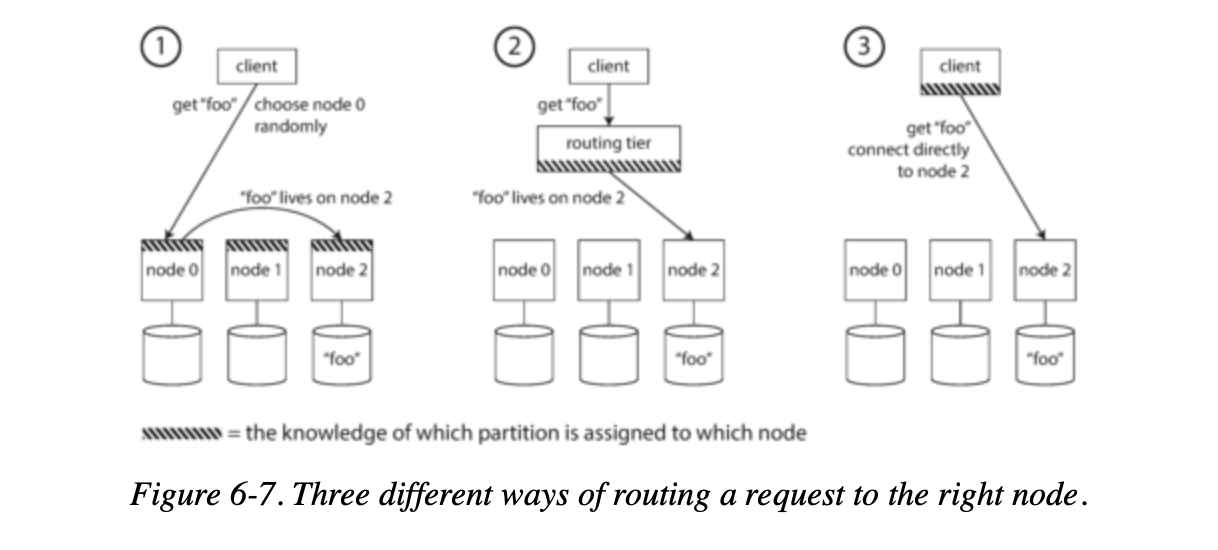
  • Allow clients to contact any node (e.g., via a round-robin load balancer).
    • If that node coincidentally owns the partition to which the request applies, it can handle the request directly; otherwise, it forwards the request to the appropriate node, receives the reply, and passes the reply along to the client.
  • Send all requests from clients to a routing tier first, which determines the node that should handle each request and forwards it accordingly.
    • This routing tier does not itself handle any requests; it only acts as a partition-aware load balancer.
  • Require that clients be aware of the partitioning and the assignment of partitions to nodes.
    • In this case, a client can connect directly to the appropriate node, without any intermediary.

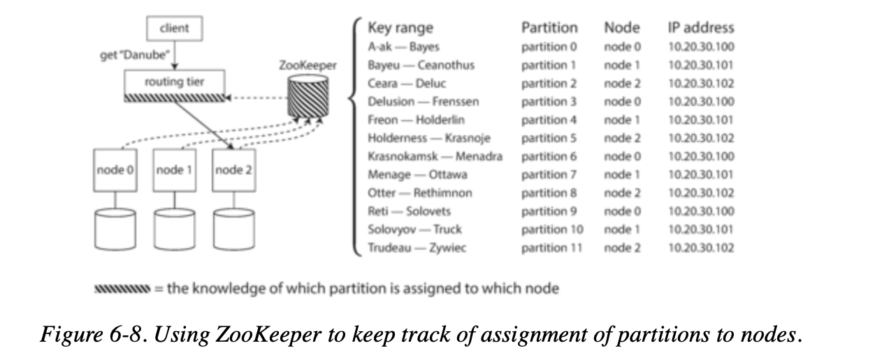
• Many distributed data systems rely on a separate coordination service such as ZooKeeper to keep track of this cluster metadata.

  • Each node registers itself in ZooKeeper, and ZooKeeper maintains the authoritative mapping of partitions to nodes.
  • Other actors, such as the routing tier or the partitioning-aware client, can subscribe to this information in ZooKeeper.
  • Whenever a partition changes ownership, or a node is added or removed, ZooKeeper notifies the routing tier so that it can keep its routing information up to date.

LinkedIn’s Espresso uses Helix for cluster management (which in turn relies on ZooKeeper). HBase, SolrCloud, and Kafka also use ZooKeeper to track partition assignment.